Guidewire Dynamics & Vascular Contact Modeling

My role: co-developer of the simulator and lead developer of the C++/Eigen mechanics backend.

Stage 01

Foundation rod mechanics

Validate rod mechanics before adding wall contact.

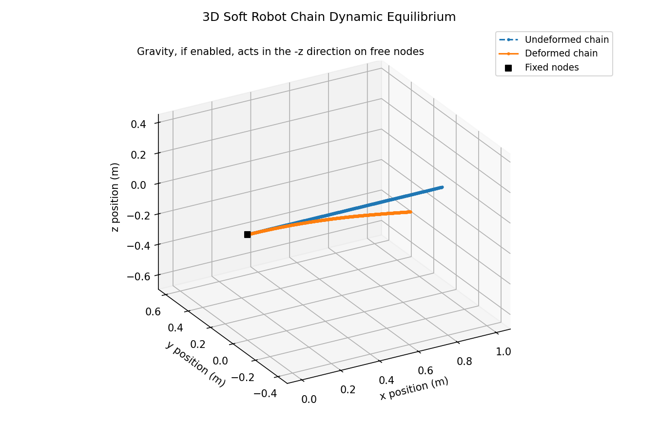
500-node cantilever under a 0.5 N tip load, showing undeformed and deformed rods in three dimensions without arrows — 500 nodes; Fy = 0.3 N, Fz = −0.4 N (0.5 N total); transverse tip displacement ≈ 303 mm. Computed static equilibrium shown at equal spatial scales; displacements are not magnified.

0.5 N: comparison with an independent nonlinear rod reference

The reference allows axial extension and large rotations without shear, matching the model's stretching and bending assumptions. All cases share the same 1 m free span, stiffness, clamp, and tip load.

Nodes	Tip difference	Relative difference
200	2.116 mm	0.689%
300	1.406 mm	0.458%
500	0.841 mm	0.274%

Result. Tip differences decrease from 0.689% to 0.458% to 0.274% as the mesh is refined. At 500 nodes, the centerline RMS difference is 0.497 mm. This is numerical agreement for one static benchmark, not measured physical accuracy.

Small-load check: 10 mN

The same independent nonlinear reference is evaluated at Fy = 6 mN and Fz = −8 mN.

Nodes	Tip difference	Relative difference
200	0.0506 mm	0.759%
300	0.0336 mm	0.504%
500	0.0201 mm	0.301%

Reference, acceptance checks, and reproduction

Counts include two fixed nodes. The free span runs from node 1 to the tip: L = 1 m, EA = 1000 N, B = 0.5 N·m², and zero gravity. Relative difference is the full 3D tip-vector difference divided by the reference tip-displacement norm. Centerlines are compared at equal undeformed material coordinates, without fitted alignment.

The independent continuum equations are solved by collocation and checked with a separate shooting method. Tightening the tolerance and changing solvers each changes reference positions by less than 10⁻⁹ m. The reference retains finite axial stiffness and excludes shear; it is not the linear small-deflection beam formula or the 500-node solution itself.

Saved rod equilibria were rechecked against the original force residual. Static minimization uses the existing rod energy, with residual-reducing Newton polishing where needed, followed by the original relaxation driver's equilibrium check. All six states pass finite-state, force, and speed gates: 10⁻⁸ N and m/s at 10 mN, and 10⁻⁶ N and m/s at 0.5 N. This is not a transient simulation from the straight state.

Reference validation records and complete comparison data and scripts include the alternative reference models. The original rod runs and plotting scripts remain available.

Stage 02

Basic PI contact

Add a protection layer near a rigid boundary, with proportional and history-dependent normal forces acting on the rod.

Planar PI-contact transient with active nodes and normal force history — A 30-node planar rod enters the wall protection layer, activating node-wise PI restoring forces. Orange markers identify active contact nodes. Vertical displacement is visually expanded. The animation loops through recorded states, slowed down rather than in real time.

Result. The recorded rod enters the protection layer and develops a normal contact response. This adds contact mechanics to the foundation model.

Demonstration conditions and numerical limits

This CPU run records 0.12 s of motion with the dynamic planar model's default rod and PI parameters. It checks finite states and nonzero protection-layer contact. It is a transient demonstration, not a settled-state, accuracy, or mesh-convergence benchmark.

The solver can stop Newton iterations on either residual or step-size tolerance. Its maximum recorded residual is 1.07 × 10⁻⁵ N, above the nominal 10⁻⁷ N residual threshold. Solver-marked convergence therefore does not mean every step passes that residual threshold.

Stage 03

Straight-tube contact

Extend contact to a three-dimensional rod inside a rigid straight tube, and track its accepted configurations under prescribed loading.

Result. The run completed 20/20 load steps; the maximum selected free-node speed was 9.52 × 10⁻⁴ m/s.

Loading conditions and acceptance checks

The 250-node case uses independent normal PI contact at nodes. Orange markers identify nodes in the protection layer; guides mark the 60 mm wall radius and 50 mm protection radius. Every animation frame is the last accepted state of its load step. The saved step-zero pulse transient is excluded.

Stage 04

Curved vessels: analytic and mesh boundaries

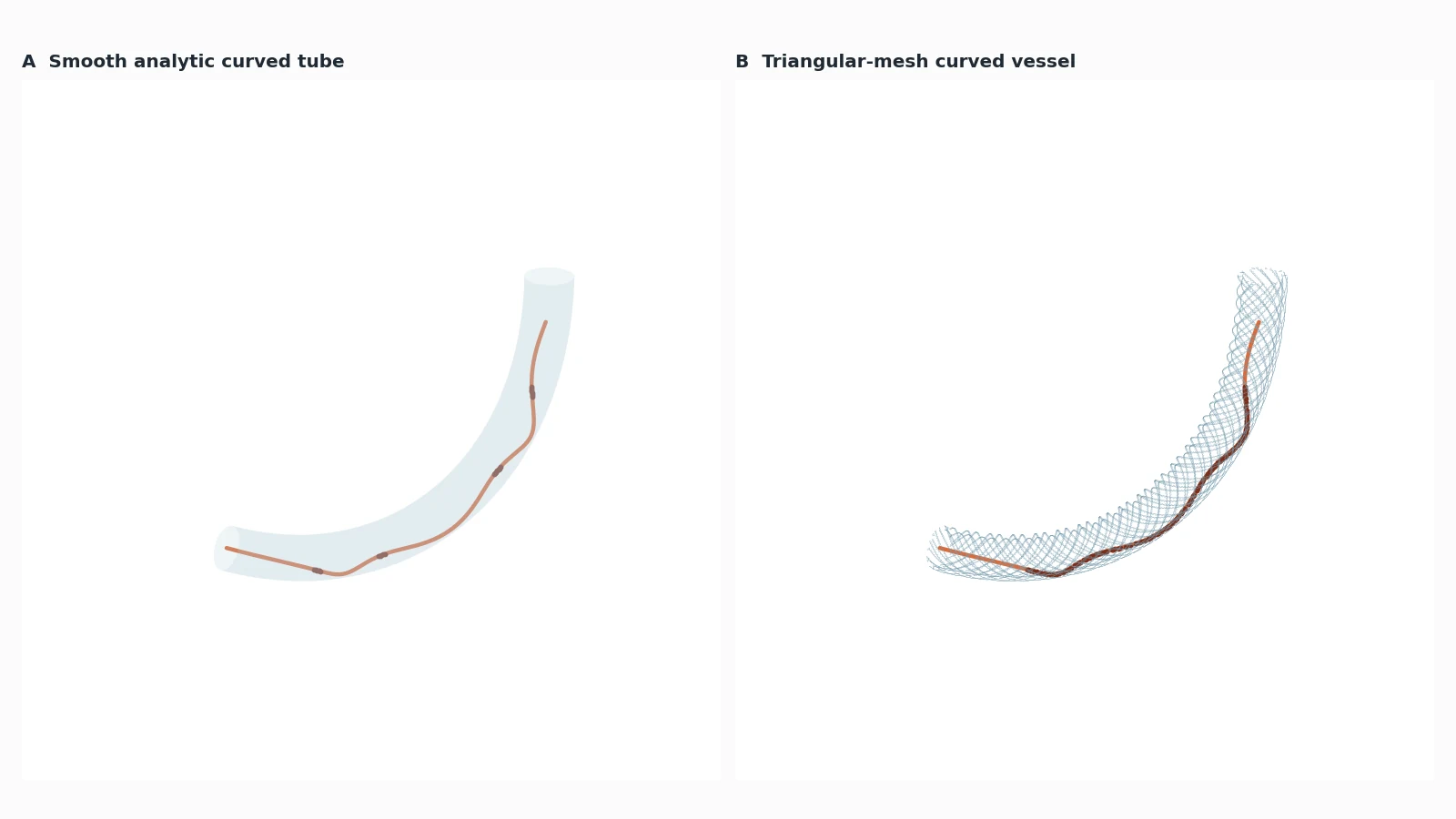
Replace the straight wall with a curved vessel and compare two descriptions of the same contact geometry.

Analytic and mesh curved-vessel contact: paired accepted states at equal prescribed displacement. The animation loops through the recorded process.

Nodewise RMS and maximum centerline position differences between analytic and mesh contact across 20 load steps — Geometry difference versus equal prescribed displacement, using corresponding node indices in the two accepted histories.

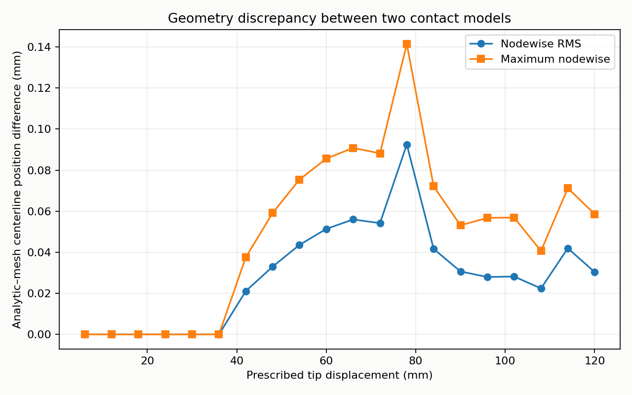
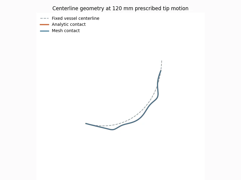
Result. Both runs completed 20/20 steps. The maximum corresponding-node difference over the accepted path was 0.141 mm, a boundary-model comparison rather than an error against physical truth.

Final configurations and matched-run conditions

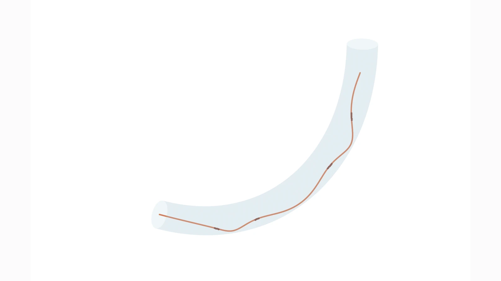
Both cases use the same 300-node rod and 120 mm loading schedule. Each displayed step passed Newton, free-node speed, contact-error, and finite-value checks. The animation uses a fixed camera and vessel-centerline reference; corresponding node indices define the differences.

Accepted final configuration of a 300-node guidewire in an analytic curved vessel — Analytic curved-vessel run, 300 nodes and 20/20 accepted load steps. This is a numerical state, not a device photograph.

Matched final analytic-boundary and mesh-boundary guidewire states — Matched curved-vessel final states. Each run passed Newton, free-node speed, contact-error, and finite-value checks at every displayed load step.

Accepted 120 mm analytic and mesh guidewire centerlines overlaid with the fixed vessel centerline — Direct centerline overlay at equal 120 mm prescribed displacement; the dashed vessel centerline fixes the spatial reference.

Stage 05

Free-end frictional insertion

Release the leading end and introduce tangential friction to examine how resistance changes the force required to advance the rod.

Free-end insertion: sampled states from matched zero- and unit-friction runs, each completing 80 loading steps. The animation loops through the recorded process.

Accepted 80-step zero- and unit-friction free-tip advance and summed axial push reaction versus imposed displacement — Matched μ = 0/1, 80-step response. Push reaction is the negative sum of axial reactions at the two prescribed actuator nodes, not pressure.

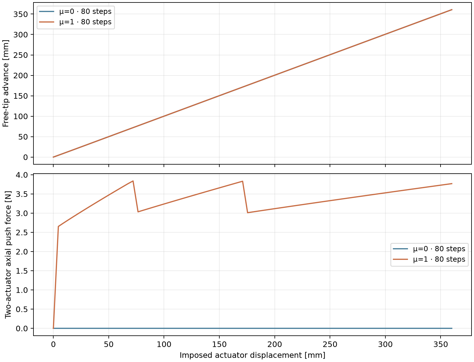
Result. At 360 mm, μ = 1 requires 3.768 N more summed push than μ = 0, while free-end advance differs by only 0.00085 mm. These records show a force response, without visually meaningful distal lag.

Boundary conditions and configuration comparison

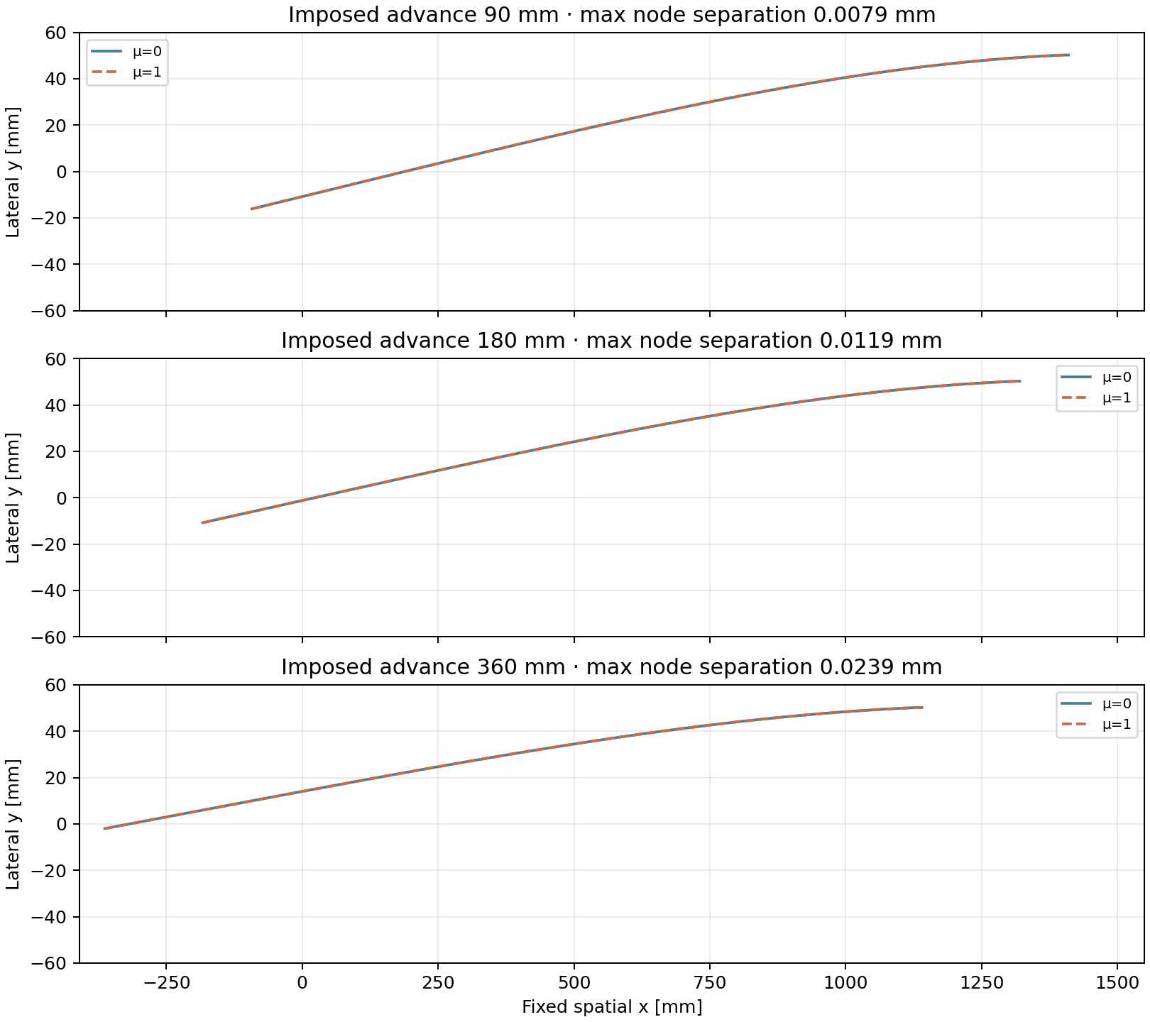
This separate three-dimensional model releases the leading end and advances two rear actuator nodes through a straight tube. The paired runs use 250 nodes and 360 mm total imposed advancement and differ only in friction coefficient, μ = 0 or 1. Both complete 80/80 steps. Their effective normal integral gain K_i changes at the same imposed displacements, 76.5 and 175.5 mm.

Push reaction is the negative sum of axial reactions at the two prescribed actuator nodes, not pressure. The largest corresponding-node separation in the final configurations is 0.024 mm.

Matched-displacement configurations for zero and unit friction at 90, 180, and 360 mm imposed advance — Configurations at matched imposed advancement, with one spatial reference for each comparison.

My contributions

I co-developed the simulator and led the C++/Eigen mechanics backend, verifying it against the Python/PyTorch reference path. I also worked on DER mechanics and derivative checks, contact and mesh-query integration, backend agreement tests, and the evidence exporters used here. The five stages above describe the project's capabilities; they are not a claim of sole authorship or a dated development timeline.

Institution: Guangdong Technion – Israel Institute of Technology
Advisor: Prof. Zhujiang Wang
Research appointment: Apr 2026 – Aug 2026

Method: elastic mechanics and implicit force balance

The untwisted rod stores stretching and bending energy, E_elastic = E_stretch + E_bend. Contact acts directly in the nonlinear residual. In PI-contact and friction runs it is not a single conservative contact-energy term. A schematic step balance is M a + C v + ∇E_elastic − F_normal − F_friction − F_external = 0, omitting terms absent from the model. Newton iterations solve each implicit step; acceptance criteria depend on the stated task.

Numerical verification & C++ backend

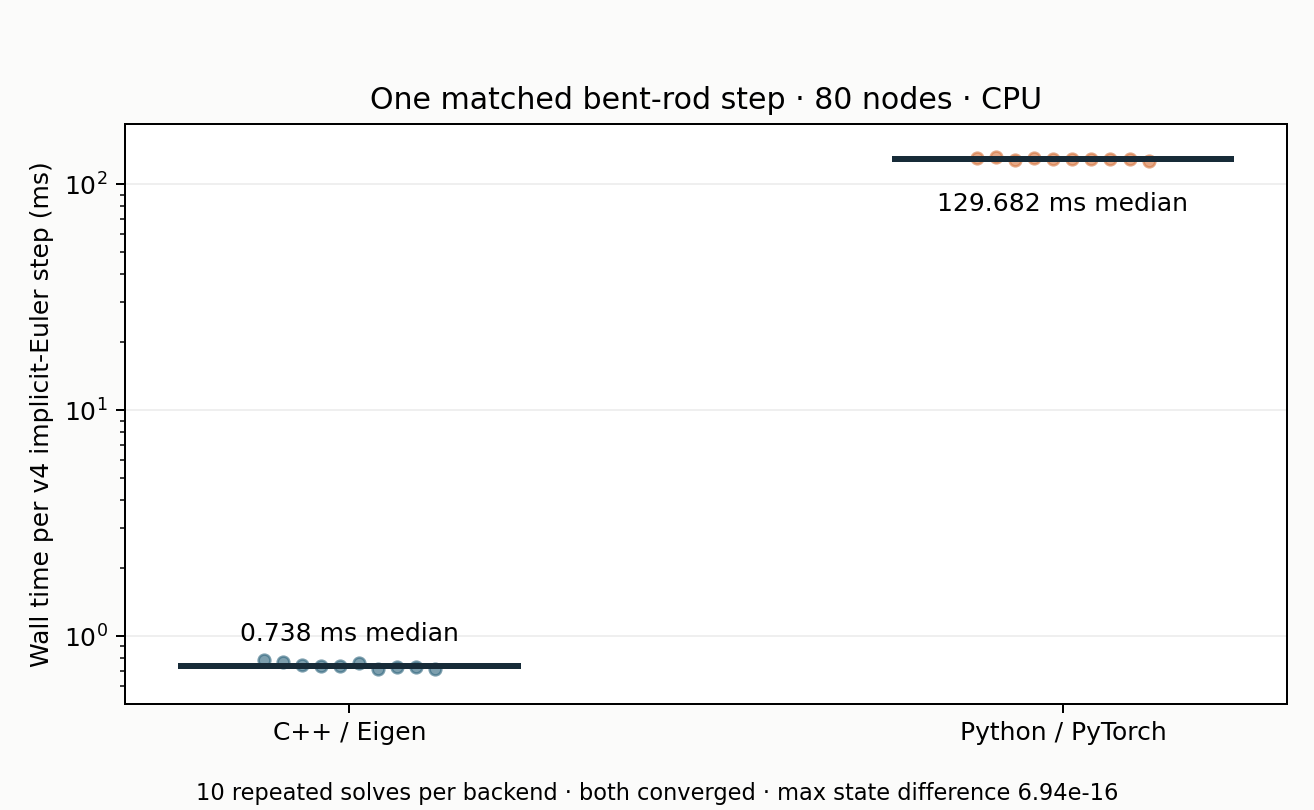
For one 80-node v4 bent-rod implicit-Euler step, Python/PyTorch and C++/Eigen both converged in 11 Newton iterations. Across ten CPU solves per backend, median wall times were 129.682 ms and 0.738 ms; the largest absolute state-field difference was 6.94 × 10⁻¹⁶. This is a single-step comparison with identical inputs and tolerances, not an end-to-end speed claim or a timing of the free-end friction model.

Ten measured CPU times per converged v4 backend with median times and maximum output difference — Matched 80-node v4 single-step timing; logarithmic time axis. Both paths passed convergence and numerical agreement gates.

Derivative verification and measurement conditions

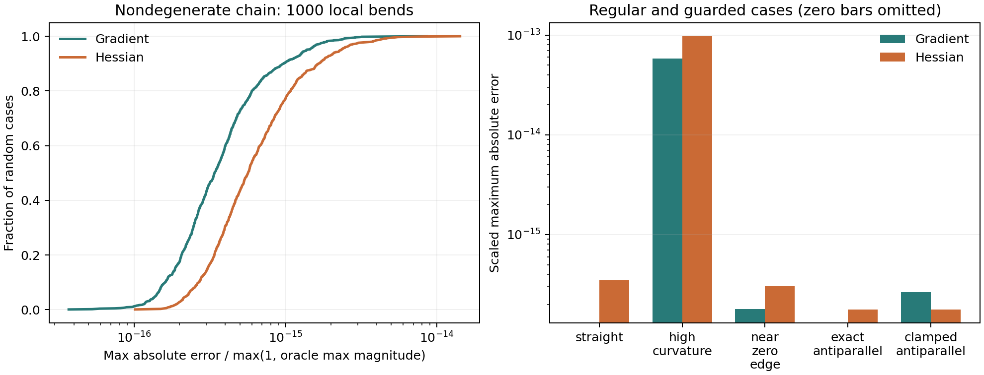
The September 2026 evidence run checked 1,000 nondegenerate local bends against a PyTorch automatic-differentiation oracle. Maximum scaled gradient and Hessian errors were 8.62 × 10⁻¹⁵ and 1.42 × 10⁻¹⁴. Straight, high-curvature, and three guarded degeneracy cases are reported separately. Timing used one thread per named BLAS/OpenMP library.

Empirical distribution of 1000 bending gradient and Hessian errors with separate guarded-branch cases — Measured derivative errors, 29 September 2026. Scaled error is maximum entrywise absolute error divided by max(1, the largest absolute oracle entry); the raw 1,005-row table and branch labels are retained in the source evidence directory.

Current limitations & next steps

The vessel walls are rigid. These models do not include flow, vessel deformation, torsional rod degrees of freedom, or physical guidewire measurements. Curved analytic/mesh comparisons use frictionless normal contact; the separate free-end model adds tangential friction.

I also developed a planar multi-bend guidewire-insertion benchmark using proximal displacement loading and Coulomb stick–slip friction. Its broader numerical campaign remains in progress and contributes no completed comparison here. For the free-end model, a node-count study awaits a defined discretization scale for normal contact parameters.

Numerical sensitivity / open issue: 80 versus 160 load steps

The full diagnostic curves below retain the individual actuator reactions and effective K_i histories.

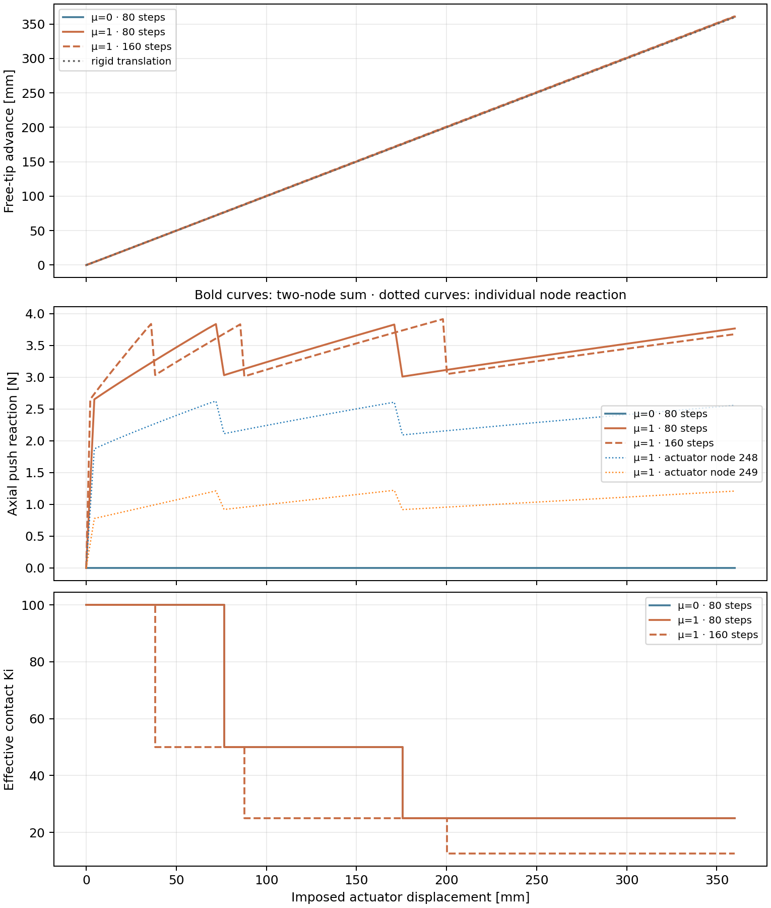
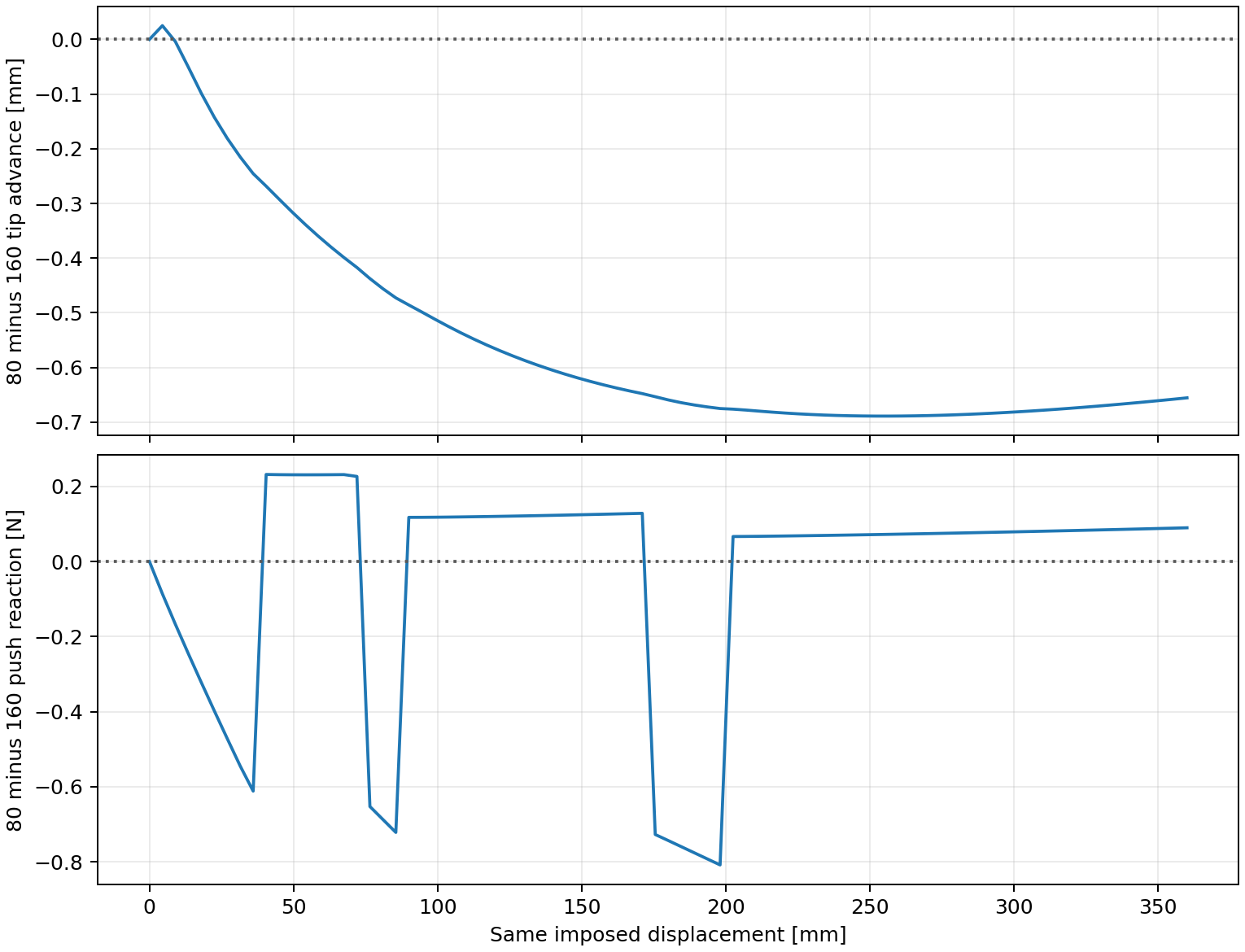
Free-end advance, individual actuator-node axial reactions, their summed push force, and effective Ki histories versus imposed advancement — Accepted 80-step μ = 0/1 and 160-step μ = 1 curves. “Push sum” is the negative sum of axial reactions at both prescribed actuator nodes; the lighter curves are individual node forces, not pressure.

A second μ = 1 run used 160 steps with the same 250 nodes, total advancement, and initial physical parameters. It completed 160/160 steps. At equal final advancement, its free-end position differs from the 80-step run by 0.656 mm and the largest corresponding-node position difference is 21.39 mm. The effective K_i schedule also changed: the 160-step path reduced it at 38.25, 87.75, and 200.25 mm. This is a loading-path sensitivity check with an adaptive-gain confound, not time integration or spatial-grid convergence.

Equal-displacement free-end advance and summed push-force differences between 80-step and 160-step friction paths — 80 minus 160 steps at matched imposed advancement; changing `K_i` histories are shown in the preceding curve figure.

Evidence & reproduction

The foundation, straight/curved vessel, friction, and backend evidence was recorded on 29 September 2026, after the research appointment. Commands, configurations, raw state hashes, requested/completed step counts, accepted-frame selection, diagnostic thresholds, and media hashes are in the original evidence index. Full raw NPZ states remain in the private research record.

The basic-contact demonstration and animation media are documented separately in the 3 October media provenance, with the contact data and reproduction script. Optimized animation sizes and frame timing are recorded in the delivery manifest and encoding scripts. The package can replay the supplied contact data independently; a fresh simulation requires the matching research source. Results establish numerical behavior for the stated cases. This evidence does not establish clinical accuracy, physical device performance, or safety.